Monte Carlo models of drug R&D focus attention on cutting costs – Part 1

There is a theme behind many of DrugBaron’s musings over the last three years: pharma R&D is just too expensive to make economic sense.  Given high failure rates throughout the process, including in particular a significant rate of late stage failures when the capital at risk is very high, either attrition must fall or costs must come down.

Almost everyone in the industry recognizes this equation.  But for most, particularly those who are guardians of large (and expensive) R&D infrastructure, it has been more palatable to talk of improving success rates than decreasing costs.

What cost cutting there has been has been quantitatively and qualitatively wrong.  Pruning a few percentage points off R&D budgets that have tripled in just a little over a decade has no discernible impact on the overall economics of drug discovery and development.  And cutting costs by reducing the number of projects, rather than reducing the cost per project, is not only ineffective but counter-productive as DrugBaron has already noted, on more than one occasion.

But there is a fundamental tension in the equation: success rates are assumed to be heavily tied to expenditure.  If you spend less per project, attrition rates will go up (assuming at least a proportion of the money is being wisely spent) and you will not improve the overall economics.  You might even make it worse.

So what makes DrugBaron so confident that dramatically cutting the cost per project makes sense? That even if decision quality declines slightly, it will be offset by a greater gain in productivity?

The “evidence” comes from sophisticated computer simulations of early stage drug development that underpin the ‘asset-centric’ investment model at Index Ventures.  Models that have remained unpublished – until now.

Drug development is a stochastic process.  That much is indisputable, given the level of failure.  Processes that we understand and control fail rarely, if ever.  But such is the complexity of biology that even the parts we think we understand relatively well still conceal secrets that can de-rail a drug development program at the last hurdle.

The fundamental premise of drug discovery and development is therefore one of sequential de-risking.  Each activity costs money and removes risk, so that the final step (usually substantial pivotal clinical trials that test whether a drug safely treats a particular disease) is positive as often as possible.

Exactly how often this last step IS positive is open to some debate.   A figure often cited for the phase 3 success rate is 50%.  But this headline figure masks considerably heterogeneity.  For example, once a drug has been shown to be effective, it is usually entered into huge programs of Phase 3 trials to provide information to support its competitive position and to expand its label, both around the initial indication and into other related indications.  Such trials are fundamentally more likely to be positive than a first phase 3 trial of any agent.  Since agents that score failures in their first couple of phase 3 trials are likely to be scratched, there is a substantial bias in favour of positive trials in the dataset as a whole.

Equally importantly, a considerable fraction of all active drug development programs can be characterized as “me too” or “me better” – in other words, modulating a target that has already been validated in earlier successful phase 3 trials (albeit with a different agent).  This eliminates most of the risk arising from the sheer complexity of biology, which remains the hardest risk to discharge in drug development.  Once again, therefore, such trials are fundamentally more likely to be positive than a first phase 3 trial of a truly “first in class” agent.

DrugBaron’s own count-back over the last five years suggests the success rate for these first phase 3 studies with agents targeting a previously unproven mechanism of action is somewhat less than 25% (unfortunately, such analysis still requires a degree of subjectivity in assigning trials into each category).

Irrespective of the precise number, the point is clear: despite best efforts to de-risk late stage trials, the majority of the risk is still there until the very end.  The drug discovery and development process, therefore, more closely resembles weather forecasting than engineering.  The contribution of stochastic processes (things which are either random or simply too complex to be properly understood at the present time) is significant – and ignored at your peril.

The take-home message is black and white: reducing cost per project is the most effective way to increase drug R&D productivity – even if it slightly damages the quality of decision-making

The time-honoured modeling algorithm for such stochastic processes is the Monte Carlo simulation.  This is a method that relies on repeated random sampling to obtain numerical estimates (in other words running simulations many times over in order to calculate those same probabilities heuristically just like actually playing and recording your results in a real casino situation: hence the name).

Our model examines a set of ‘projects’ with defined characteristics (explained below) taken from concept through to phase 2a clinical proof-of-concept.   The output assigns a cost to each action taken in each project, and attributes a value to each positive clinical proof of concept study.  While our intention was to model an early stage venture fund (with a portfolio of such projects), the lessons apply equally to any institution running multiple drug discovery and early development projects, such as pharma companies.  There is nothing in the model that intrinsically relates to a venture fund.

The key to the model is the concept of the ‘action-decision chain’ – the principle that even something as complex as drug discovery and development can be reduced to a sequence of actions (experiments that generate data) followed by a decision as to whether to kill or continue the project to the next stage.  It doesn’t much matter what sort of data is envisaged (ADME, toxicology, efficacy, CMC, clinical and so forth), the process is entirely generic – you collect the data, examine it and make your decision.

Each action, in the model, has only one parameter: cost.  At each stage, you can spend a little or a lot (which presumably affects the amount and quality of the data that you obtain).  The model doesn’t attempt to characterize what the individual steps are, but merely assumes that each successive step is more costly than the last one (which, if you are doing your drug development right it should be – you should discharge the cheapest risks first).

The way each decision point is modeled is critical to the output.  The model has an internal flag (set at the beginning of each run) as to whether that agent ‘works’ or not.  This is the real world situation: the day you decide to develop a particular molecule for a particular indication, the dice has been rolled: it either does work in that indication or not – its just that you won’t know for many years, and many millions of dollars!

At each decision point, then, a filter is applied that has a false positive rate (that is, the data looks fine, so the management continue even though actually the project is doomed to eventually fail) and a false negative rate (where the management kill a project that would, had they continued, actually been successful).  If you set all the decision filters to have perfect quality (no false negatives and no false positives) then only successful projects are progressed and productivity is maximized.  But to model the real world, you can introduce imperfect decision-making at different levels (and with different emphasis on false positives versus false negatives – a parameter we call ‘stringency’ of decision making: complete stringency would mean that all projects are killed; 100% false negative rate but 0% false positive rate).

The computer then runs all the projects, and calculates the total amount spent on all the actions across all the projects (and, of course, as soon as a project is ‘killed’ it ceases to progress to the next, more expensive, action).  At the end, when every live program has read out its phase 2a proof of clinical concept, the model sums up the value that has been created.  The output is a return on capital invested.

Of course, because of the random element modeled in the decision-making (the non-zero false negative and false-positive rates), every time the simulation is run on a collection of projects, with all the parameters set the same, there will be a different global outcome (the return on capital will vary, depending by chance how often the decision filters ‘got it right’ in that run).

As a result, to get an estimate of how “good” that set of parameters really are, the simulation is run a hundred times on a hundred different sets of projects.  This allows the mean return of capital if you operating under those conditions of cost and decision quality to be estimated (as well, interestingly, as the standard deviation of the returns between runs).

And so to the results!

The base conditions for the model assumed 10% of the projects were inherently ‘working’ when setting the hidden flag.  Of these 50% of the failures were eliminated as obvious (simulating the process by which a venture investor or pharma committee screens candidate projects and decides whether to initiate them or not).  Thereafter, the remainder began a series of action-decision steps, with €1m spent prior into initiating development, €5m spent on formal preclinical and phase 1 and €10m spent on Phase 2 proof of concept.  The actual sums spent don’t really matter because the output depends on the arbitrarily assigned value of a successful proof-of-concept (its only the ratio of the value created to the amount spent which is interesting).  If you are a pharma company, rather than a cash-conscious asset-centric investment fund, you may want to add a zero to each of the above.

In the base model, the filter was set with a 33% false-positive rate (so that ‘only’ 66% of the real failures are stopped at each stage), and a 10% false-negative rate (wrongly stopping 10% of the real successes).

At the end, each of the real successes (based on the hidden flag) that are still alive is attributed a 50% chance of being sold for €50m (simulating an exit for the venture fund – if you were modeling the same processes in a pharma company, for example, you may select a different estimate of output value, or more likely, choose to carry the simulation beyond Phase 2 proof of clinical concept).

 

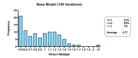
With these parameters, the median fund returns 0.77 of the capital invested, with fully 63% of such funds losing money.  Only 3% of funds returned more than 1.5x invested capital.  That may be weaker than real-world performance – it is certainly much worse than the Index Ventures track record – but the arbitrary selection of exit values means that the absolute returns are not what is interesting.  The real interest comes from examining the relative impact of changing the model parameters.  How does altering the cost of R&D, or the quality and stringency of decision-making affect returns?

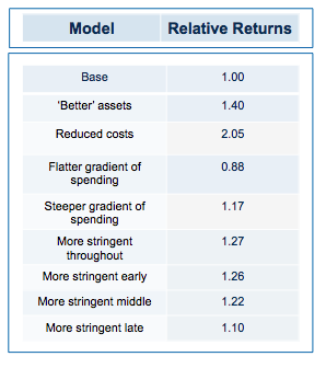
Obviously, if you run the simulation with a slightly higher quality of asset in the initial pool, returns are increased (doubling asset quality, so that 20% of the assets have their hidden flag marked as successful, increases median returns but only to 1.1 fold).  Returns, then, are not principally determined by how many pearls there are in the swamp.

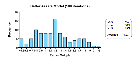
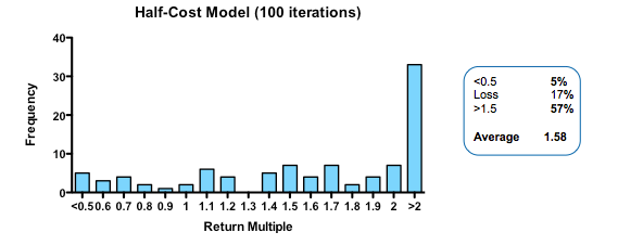
By contrast, cutting costs translate linearly into improved returns.  Halving the amount paid for each action-decision pair, yields a median return of 1.58 fold, with fully one third of funds returning over 2x (compared with only 3% passing this threshold in the base model).

Plotting return against the relative cost for each action-decision pair reveals two interesting phenomena: first, the gain in returns is slightly better than linear across the whole cost range, with particularly spectacular benefits when the cost becomes much smaller than the average value of the successful exit.  Second, and less intuitively, the standard deviation of returns across a hundred iterations of the same fund parameters declines as cost goes down.  In other words, not only are median returns increasing, but the chances of getting a return close to median is also increased (which should comfort real-world investors who have only one, or a small number, of funds to worry about at any given moment).

More subtle models, varying not the total expenditure but when it is spent (in other words the gradient by which costs increase with each sequential action-decision pair) show that keeping early spending low is the critical parameter for improving returns.  This makes sense: at the beginning, the team is operating in the least data-rich environment, so making decisions virtually in the dark has a large element of random chance.  As data accumulates, the ability to make decisions improves (and, assuming sequential de-risking has been taking place, the average quality of the asset pool still alive is also increasing).  As DrugBaron has noted before, the important thing is that capital at risk is graded as steeply as possible from low to high as a project progresses.

So much for costs.  What about decision quality?

The parameters that control the decision filter (false-negative rate and false-positive rate) can be tweaked in two different ways: they can be altered so that the decision quality improves (that is, that more decisions are objectively correct compared to the hidden flag) or that the stringency increases (for the same quality of decision making, the decision is more likely to be a kill).

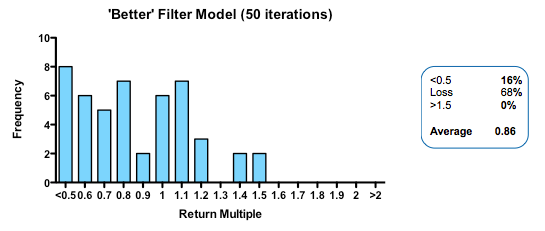
Strikingly, a four-fold improvement in filter quality (achieved by halving the rate of both the false-negative and false-positive parameters) had only a marginal benefit on returns (median 0.86 fold versus 0.77 in the base model).  In fact, once the decision quality reaches a point where at least 2 out of 3 decisions are objectively correct, then returns hardly increase at all beyond that point.

In the part of the curve where we operate in the real world (with something of a majority of correct decisions), the model tells us that returns are very insensitive to further improvements in the decision-making quality.  The reason for this is simple: because early decisions have to be made on the basis of very little data (the model, like real-world early stage drug developers, is operating in what Daniel Kahneman called a ‘low validity environment’) random chance is as important as the ability to make decisions based on the data that has been revealed up until that point.

Now for the critical ‘experiment’: tying together the quality of the filter with the amount paid of each action (simulating the widely-held view that the more we spend on drug discovery the better the dataset we accumulate on which to make decisions).  And the answer?  Assuming the decision quality is at least 60% correct decisions, then it NEVER pays to spend more in order to increase the quality of the decision filter.  In other words, the productivity gain from the improved decision filter is more than offset by the productivity loss from the increase in capital at risk.

Of course, like any simulation, these mathematical Monte Carlo models are an imperfect surrogate for the complex world of drug discovery and development.  The simplifications made are manifold (not least that all types of data provide the same contribution to decision quality per dollar they cost to obtain, which is unlikely to be true).  Moreover, the very structure of the model enshrines the principle of “working in the dark” at the start of the process and gradually gaining more visibility on the ‘real’ outcome as the process continues – in other words the idea that drug development as a process has substantial stochastic component.

At every stage of the drug development process there is more that you don’t know than you do know – ignore that at your peril

But once you accept the stochastic component is material (which current failure rates, even in phase 3, surely support), then the lessons these models teach us are likely to have some value, even if they should not be literally translated into a rigid new framework for drug development.  And those lessons are simple: spend as little as possible on as many unrelated projects as possible; apply a highly stringent filter, but do not pay ‘extra’ to try and improve the quality of the decision filter; and above all focus on reducing costs per project.

If that sounds familiar, that is no accident.  The insights from these models underpin the “kill the losers” strategy at the heart of asset-centric investing (as well as the antipathy towards a “pick the winners” strategy).  As real-world evidence starts to accumulate that supports the predictions from the model – as the recent paper from The Boston Consulting Group in Nature Biotechnology certainly does – then our confidence in putting these lessons into practice will only grow.

 

Cutting costs in pharma R&D comes with a caveat, however: read it here in Part 2